本文对Advice for applying Machine Learning一文中提到的算法诊断等理论方法进行实践,使用Python工具,具体包括数据的可视化(data visualizing)、模型选择(choosing a machine learning method suitable for the problem at hand)、过拟合和欠拟合识别和处理(identifying and dealing with over and underfitting)、大数据集处理(dealing with large datasets)以及不同代价函数(pros and cons of different loss functions)优缺点等。
数据可视化
数据集获取
使用\(sklearn\)自带的\(make\_classification\)方法获取数据。
1 | from sklearn.datasets import make_classification |
我们对二分类问题进行讨论,选取了1000个样本,20个特征。下表是部分数据: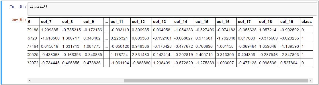
显然尽管维度很少,直接看这个数据很难得到关于问题的任何有用信息。我们通过可视化数据来发现规律。
可视化
我们使用\(Seaborn\)开源库来进行可视化。
第一步我们使用pairplot方法来绘制任意两个维度和类别的关系,我们使用前100个数据,5个维度特征来进行绘图。1
_ = sns.pairplot(df[:100], vars=["col_8", "col_11", "col_12", "col_14", "col_19"], hue="class", size=1.5)
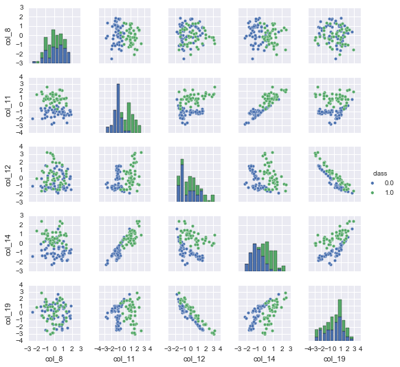
上图25幅图,是5个维度特征两两组合的结果。对角线的柱状图反映了同一个维度不同类别之间取值的差异,从图中可以看出特征11和特征14取值在不同类别间差异显著。再观察散点图,散点图反映了任意两个维度组合特征和类别的关系,我们可以根据是否线性可分或者是否存在明显的相关来判断组合特征在类别判断中是否起到作用。如图特征11和特征14的散点图,我们发现基本上是线性可分的,而特征12和特征19则存在明显的反相关。对于相关性强的特征我们必须舍弃其一,对于和类别相关性强的特征必须保留。
我们继续观察特征与特征之间以及特征与类别之间的相关性:1
2
3plt.figure(figsize=(12, 10))
plt.xticks(rotation=90)
_ = sns.heatmap(df.corr()) #df.corr()是求相关系数函数
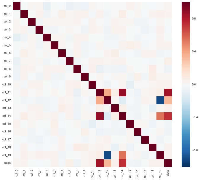
如上图,我们使用热力图来绘制不同特征之间以及特征与类别之间的相关性。首先看最后一行,反映了类别和不同特征之间的关系。可以看到,特征11和类别关系最密切,即特征11在类别判断中能起到很重要的作用。特征14、12次之。再看特征12和特征19,我们发现存在着明显的反相关,特征11和特征14正相关性也很强。因此存在一些冗余的特征。因为我们很多模型是假设在给定类别的情况下,特征取值之间是独立的,比如朴素贝叶斯。而剩余的其他特征大部分是噪声,既和其他特征不相关,也和类别不相关。
模型初步选择
一旦我们对数据进行可视化完,就可以快速使用模型来进行粗糙的学习(回顾前文提到的bulid-and-fixed方法)。由于机器学习模型多样,有的时候很难决定先用哪一种方法,根据一些总结的经验,我们使用如下图谱入手:1
2from IPython.display import Image
Image(filename='machine-learning-method.png', width=800, height=600)
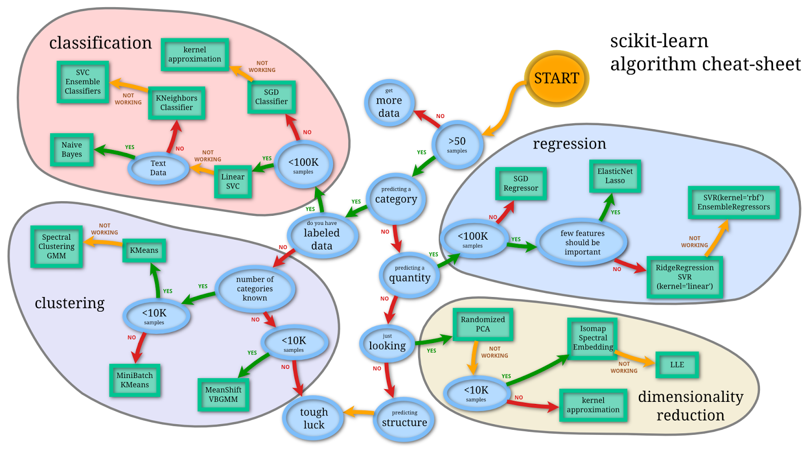
因为我们有1000个样本,并且是有监督分类问题,根据图谱推荐使用\(LinearSVC\),我们首先使用线性核函数的SVM来尝试建模。回顾一下\(SVM\)的目标函数:
$$\min_{\gamma,w,b} \frac{1}{2}{||w||}^2+C \sum_{i=1}^m \zeta_i \\\ 使得, y^{(i)}(w^T x^{(i)} + b) \geq 1-\zeta_i, i=1,…,m \\\ \zeta_i \geq 0, i=1,…,m$$
上式使用的是L2-regularized,L1-loss(\(C \sum_{i=1}^m \zeta_i\))(具体含义参加SVM支持向量机-软间隔分类器一节)。因此penalty=’l2’,loss=’hinge’,即:1
2
3
4
5
6#http://scikit-learn.org/stable/modules/generated/sklearn.svm.LinearSVC.html
from sklearn.svm import LinearSVC
# 二者间距较大,存在过拟合的嫌疑,即训练集拟合的很好,分数很高。但是测试集分数很低
plot_learning_curve(LinearSVC(C=10.0,penalty='l2',loss='hinge'), "LinearSVC(C=10.0,penalty='l2',loss='hinge')",
X, y, ylim=(0.8, 1.01),
train_sizes=np.linspace(.05, 0.2, 5),baseline=0.9)
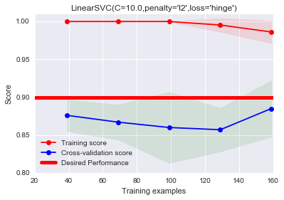
上式是学习曲线,对应我们之前提到的诊断方法中的方差/误差分析图。我们在下一小节介绍该图的细节。我们现在先关注上图,我们只使用了20%(np.linspace第二个参数),即200个数据进行训练测试。由图中可以看出,训练分数和泛化分数二者间距较大,并且训练分数处在一个很高的水准,根据之前介绍的偏差方差分析,我们可以得出,上述存在过拟合(over-fitting)的问题。注意,该学习曲线和之前偏差方差分析图存在区别: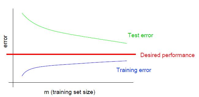
区别在于,之前使用的是误差,这里使用的是得分。因此测试集和训练集分数曲线相对位置调换,训练集分数曲线在上,测试集分数曲线在下。随着样本的增多,误差曲线下降,这里分数曲线则是上升。但是相同点在于,过拟合图对应的学习曲线,训练分数(误差)和泛化分数(误差)二者间距较大,且训练分数(误差)处在一个高水准。
学习曲线
这里我们先介绍下学习曲线绘制方法。1
2
3
4
5
6
7
8
9
10
11
12
13
14
15
16
17
18
19
20
21
22
23
24
25
26
27
28
29
30
31
32
33
34
35
36
37
38
39
40
41
42
43
44
45
46
47
48
49
50
51
52
53
54
55
56
57
58
59
60
61
62# http://scikit-learn.org/stable/modules/learning_curve.html#learning-curves
from sklearn.learning_curve import learning_curve
def plot_learning_curve(estimator, title, X, y, ylim=None, cv=None,
train_sizes=np.linspace(.1, 1.0, 5),baseline=None):
"""
Generate a simple plot of the test and traning learning curve.
Parameters
----------
estimator : object type that implements the "fit" and "predict" methods
An object of that type which is cloned for each validation.
title : string
Title for the chart.
X : array-like, shape (n_samples, n_features)
Training vector, where n_samples is the number of samples and
n_features is the number of features.
y : array-like, shape (n_samples) or (n_samples, n_features), optional
Target relative to X for classification or regression;
None for unsupervised learning.
ylim : tuple, shape (ymin, ymax), optional
Defines minimum and maximum yvalues plotted.
cv : integer, cross-validation generator, optional
If an integer is passed, it is the number of folds (defaults to 3).
Specific cross-validation objects can be passed, see
sklearn.cross_validation module for the list of possible objects
"""
plt.figure()
train_sizes, train_scores, test_scores = learning_curve(
estimator, X, y, cv=5, n_jobs=1, train_sizes=train_sizes)
print train_sizes
print '-------------'
print train_scores
train_scores_mean = np.mean(train_scores, axis=1)
train_scores_std = np.std(train_scores, axis=1)
test_scores_mean = np.mean(test_scores, axis=1)
test_scores_std = np.std(test_scores, axis=1)
plt.fill_between(train_sizes, train_scores_mean - train_scores_std,
train_scores_mean + train_scores_std, alpha=0.1,
color="r")
plt.fill_between(train_sizes, test_scores_mean - test_scores_std,
test_scores_mean + test_scores_std, alpha=0.1, color="g")
plt.plot(train_sizes, train_scores_mean, 'o-', color="r",
label="Training score")
plt.plot(train_sizes, test_scores_mean, 'o-', color="b",
label="Cross-validation score")
if baseline:
plt.axhline(y=baseline,color='red',linewidth=5,label='Desired Performance') #baseline
plt.xlabel("Training examples")
plt.ylabel("Score")
plt.legend(loc="best")
plt.grid("on")
if ylim:
plt.ylim(ylim)
plt.title(title)
简要解释下几个重要点。首先是参数,estimator代表模型,title标题,X是样本数据集,y是标签集,ylim是学习曲线y轴的取值范围(min,max),cv是交叉验证折数,train_sizes=np.linspace(.1, 1.0, 5)代表划分训练集,np.linspace(.1, 1.0, 5)返回的结果[ 0.1 , 0.325, 0.55 , 0.775, 1. ],即等间隔划分数据集,第一个参数是起始,第二个参数是终点,最后一个参数是划分份数。因为学习曲线的x轴代表样本的数量,即画出指标在训练集和验证集上样本数量变化的情况。我们不可能对每个样本量取值(从1一直递增到1000)都进行绘图,即不能画出平滑的曲线,而是取一些关键的点进行训练绘图,上述得到的train_sizes就是每次训练的样本占总样本的比例的数组。
接着是重要的一些代码。train_sizes, train_scores, test_scores = learning_curve(estimator, X, y, cv=5, n_jobs=1, train_sizes=train_sizes)返回的train_sizes是根据传入的train_sizes比例数组计算的实际训练样本数量数组。train_scores是训练集的得分,是一个二维数组,第一维等于train_sizes数组大小,即每次训练的分数,第二维等于交叉验证份数cv,即每次交叉验证的得分数组。test_scores是测试集的得分。因此可以取平均进行绘图,plt.fill_between方法是图中阴影的部分。
过拟合处理
有许多方法可以解决过拟合问题。
增加样本数量
1 | plot_learning_curve(LinearSVC(C=10.0,penalty='l2',loss='hinge'), "LinearSVC(C=10.0,penalty='l2',loss='hinge')", |
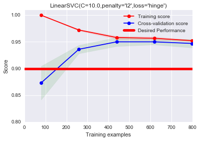
这里修改linspace第二个参数为1,使用全部样本进行训练。我们发现泛化分数随着样本的增多不断增大,并且泛化分数和训练分数的间距不断缩小。但是高偏差的时候间距也是小的,我们继续进一步判断,发现训练分数和泛化分数都处在一个较高的水准,高于期望分数,而高偏差时,训练分数和泛化分数都比较低,低于理想分数。因此此时不存在过拟合或欠拟合的问题。
减少特征
根据前面的可视化分析,我们发现特征11和14和类别关联紧密,因此可以考虑先手动选择这两种特征进行训练。同样只在20%的样本上进行训练:1
2
3plot_learning_curve(LinearSVC(C=10.0,penalty='l2',loss='hinge'), "LinearSVC(C=10.0,penalty='l2',loss='hinge') Features: 11&14",
df[["col_11", "col_14"]], y, ylim=(0.8, 1.0),
train_sizes=np.linspace(.05, 0.2, 5),baseline=0.9)
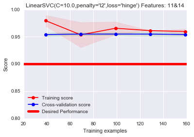
和最早的那幅过拟合图相比,这里的结果已经好很多,基本上解决了过拟合的问题。但是这里的特征选择方法有点作弊嫌疑,首先是因为手动选择的,其次是因为我们是在1000个样本上进行选择的,而我们最终却只使用200个样本进行训练绘图。下面进行特征自动选择:1
2
3
4
5
6
7
8from sklearn.pipeline import Pipeline
from sklearn.feature_selection import SelectKBest, f_classif
# SelectKBest(f_classif, k=2) will select the k=2 best features according to their Anova F-value
plot_learning_curve(Pipeline([("fs", SelectKBest(f_classif, k=2)), # select two features
("svc", LinearSVC(C=10.0,penalty='l2',loss='hinge'))]),
"SelectKBest(f_classif, k=2) + LinearSVC(C=10.0,penalty='l2',loss='hinge')",
X, y, ylim=(0.8, 1.0),
train_sizes=np.linspace(.05, 0.2, 5),baseline=0.9)
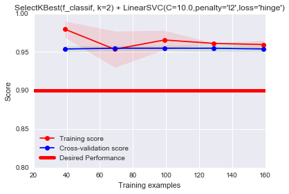
上述使用\(SelectKBest\)选择2个特征,我们发现在这个数据集上特征选择表现很好。注意,这种特征选择方法只是减少模型复杂度的一种方法。其他方法还包括,减少线性回归中多项式的阶数,减少神经网络中隐藏层的数量和节点数,增加高斯核函数的bandwidth(\(\sigma\)),或减小\(\gamma\)等(参考SVM C和gamma参数理解)。
修改目标函数正则化项
1 | #C表征了对离群点的重视程度,越大越重视,越大越容易过拟合。 |
惩罚因子\(C\)决定了你有多重视离群点带来的损失,显然当所有离群点的松弛变量(\(\zeta\))的和一定时,你定的C越大,对目标函数的损失也越大,此时就暗示着你非常不愿意放弃这些离群点,最极端的情况是你把C定为无限大,这样只要稍有一个点离群,目标函数的值马上变成无限大,马上让问题变成无解,这就退化成了硬间隔问题,即C越大,你越希望在训练数据上少犯错误,而实际上这是不可能/没有意义的,于是就造成过拟合。
因此这里减少\(C\)能够一定程度上减少过拟合。
我们可以使用网格搜索来寻找最佳C。1
2
3
4
5
6
7
8#使用网格搜索
from sklearn.grid_search import GridSearchCV
est = GridSearchCV(LinearSVC(penalty='l2',loss='hinge'),
param_grid={"C": [0.0001,0.001, 0.01, 0.1, 1.0, 10.0]})
plot_learning_curve(est, "LinearSVC(C=AUTO)",
X, y, ylim=(0.8, 1.0),
train_sizes=np.linspace(.05, 0.2, 5),baseline=0.9)
print "Chosen parameter on 100 datapoints: %s" % est.fit(X[:100], y[:100]).best_params_
输出结果:Chosen parameter on 100 datapoints: {‘C’: 0.01}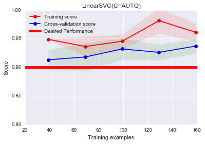
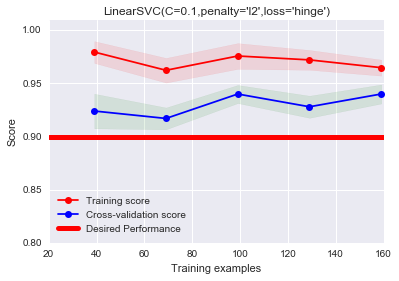
特征选择看起来比修改正则化系数来的好。还有一种正则化方法,将LinearSVC的penalty设置为L1,官方文档解释为The ‘l1’ leads to coef_ vectors that are sparse,即L1可以导致稀疏参数矩阵,参数为0的特征不起作用,则相当于隐含的特征选择。不过注意,LinearSVC不支持L1-regularized和L1-loss,L1-regularized对应penalty=’l1’,L1-loss对应loss=’hinge’。可参考Liblinear does not support L1-regularized L1-loss ( hinge loss ) support vector classification. Why?因此需要把loss改成’squared_hinge’。另外,此时不能用对偶问题来解决。故dual=False。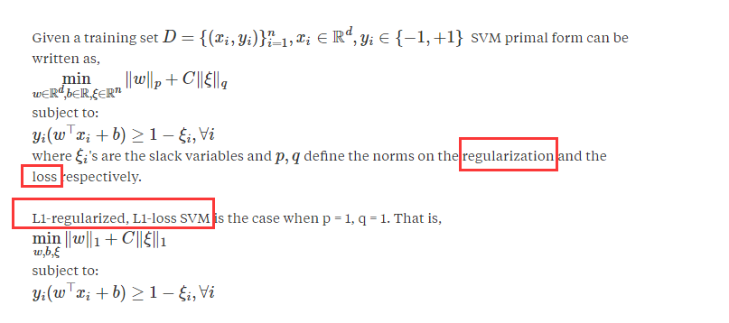
1
2
3
4plot_learning_curve(LinearSVC(C=0.1, penalty='l1', loss='squared_hinge',dual=False),
"LinearSVC(C=0.1, penalty='l1')",
X, y, ylim=(0.8, 1.0),
train_sizes=np.linspace(.05, 0.2, 5),baseline=0.9)
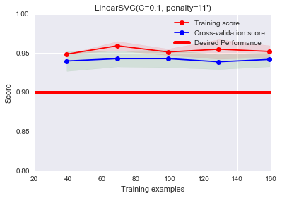
结果看起来不错。
学习到的参数如下:1
2
3
4est = LinearSVC(C=0.1, penalty='l1', loss='squared_hinge',dual=False)
est.fit(X[:150], y[:150]) # fit on 150 datapoints
print "Coefficients learned: %s" % est.coef_
print "Non-zero coefficients: %s" % np.nonzero(est.coef_)[1]
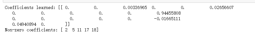
可以看到特征11的权重最大,即最重要。
欠拟合处理
之前使用的数据集分类结果都比较理想,我们尝试使用另一个二分类数据集。1
2
3
4
5from sklearn.datasets import make_circles
X, y = make_circles(n_samples=1000, random_state=2)#只有2个特征
plot_learning_curve(LinearSVC(C=0.25), "LinearSVC(C=0.25)",
X, y, ylim=(0.4, 1.0),
train_sizes=np.linspace(.1, 1.0, 5))#效果非常差
由上图可以看出,训练分数和泛化分数差距很小,并且训练分数明显低于期望分数。根据之前的方差/偏差分析可知,这里存在着明显的偏差,即欠拟合问题。
我们首先对数据进行可视化观察:1
2
3
4
5# 环形数据,外圈的数据是一种类别,内圈的数据是一种类别
columns = map(lambda i:"col_"+ str(i),range(2)) + ["class"]
df = DataFrame(np.hstack((X, y[:, None])),
columns = columns)
_ = sns.pairplot(df, vars=["col_0", "col_1"], hue="class", size=3.5)
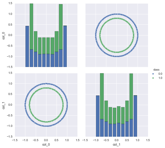
根据上图,该数据集是环形数据,外圈的点代表一种类别,内圈的点代表另一种类别。显然上述数据是线性不可分的,使用再多数据或者减少特征都没用,我们的模型是错误的,需要进行欠拟合处理。
增加或使用更好的特征
我们尝试增加特征,根据散点图,显然不同类别距离原点的距离不同,我们可以增加到原点的距离这一特征。1
2
3
4
5
6#解决欠拟合方法1:增加特征
# X[:, [0]]**2 + X[:, [1]]**2)计算的是离原点的距离
X_orginal_distance = X[:, [0]]**2 + X[:, [1]]**2#X[:, [0]]将得到的列数据变成二维的形式,[[ 8.93841424e-01],[ -7.63891636e-01]...]
df['col_3'] = X_orginal_distance
#可以看到完全线性可分
_ = sns.pairplot(df, vars=["col_0", "col_1","col_3"], hue="class", size=3.5)
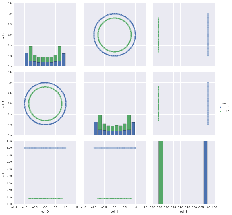
由最后一幅图,我们发现根据col_3新特征,就能将类别完全线性分隔开,因此col_3特征在区分类别上能起决定性作用。不妨看看热力图: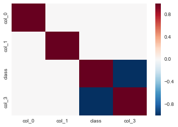
根据热力图,我们发现col_3和类别存在着非常强的负相关性。使用新增完的特征集进行预测:1
2
3
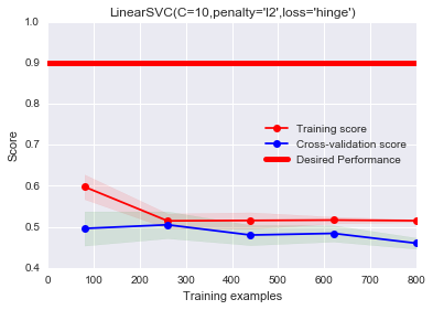
4X_extra = np.hstack((X,X[:,[0]]**2+X[:,[1]]**2))
plot_learning_curve(LinearSVC(C=10,penalty='l2',loss='hinge'), "LinearSVC(C=10,penalty='l2',loss='hinge')",
X_extra, y, ylim=(0, 1.01),
train_sizes=np.linspace(.1, 1.0, 5),baseline=0.9)
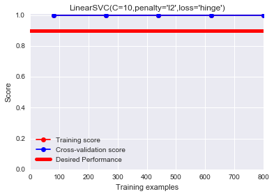
根据结果,完全分开了样本。我们可以进一步思考,是否可以让模型进行自动生成新特征?
使用更复杂的模型
使用复杂的模型,相当于更换了目标函数。根据上面数据集非线性可分的特点,我们可尝试非线性分类器,使用RBF核的SVM进行分类。1
2
3
4
5
6
7from sklearn.svm import SVC
# note: we use the original X without the extra feature
# 使用RBF核,最小间隔gamma设为1.
plot_learning_curve(SVC(C=10, kernel="rbf", gamma=1.0),
"SVC(C=10, kernel='rbf', gamma=1.0)",
X, y, ylim=(0.5, 1.1),
train_sizes=np.linspace(.1, 1.0, 5),baseline=0.9)
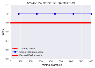
注意上述建模使用的是原始数据集X,而没有用新的特征。可以发现结果很理想,RBF核会将特征映射到高维空间,因此得到的非线性模型效果很好。
大数据集和高维特征处理
SGDClassfier增量学习
如果数据集增大,特征增多,那么上述SVM运行会变慢很多。根据之前的图谱推荐,此时可以使用\(SGDClassifier\),该分类器也是一个线性模型,但是使用随机梯度下降法(stochastic gradient descent),\(SGDClassifier\)对特征缩放很敏感,因此可以考虑标准化数据集,使特征均值为0,方差为1.
\(SGDClassifier\)允许增量学习,会在线学习,在数据量很大的时候很有用。此时不适合采用交叉验证,我们采取progressive validation方法,即将数据集等分成块,每次在前一块训练,在后一块验证,并且使用增量学习,后面块的学习是在前面块学习的基础上继续学习的。
首先生成数据,20万+200特征+10个类别。 1
2
3X, y = make_classification(200000, n_features=200, n_informative=25,
n_redundant=0, n_classes=10, class_sep=2,
random_state=0)
建模和验证:1
2
3
4
5
6
7
8
9
10
11
12
13
14
15
16
17
18
19
20
21from sklearn.linear_model import SGDClassifier
def sgd_score(X,y):
est = SGDClassifier(penalty="l2", alpha=0.001)
progressive_validation_score = []
train_score = []
for datapoint in range(0, 199000, 1000):
X_batch = X[datapoint:datapoint+1000]
y_batch = y[datapoint:datapoint+1000]
if datapoint > 0:
progressive_validation_score.append(est.score(X_batch, y_batch))
est.partial_fit(X_batch, y_batch, classes=range(10)) #增量学习或称为在线学习
if datapoint > 0:
train_score.append(est.score(X_batch, y_batch))
plt.plot(train_score, label="train score",color='blue')
plt.plot(progressive_validation_score, label="progressive validation score",color='red')
plt.xlabel("Mini-batch")
plt.ylabel("Score")
plt.axhline(y=0.8,color='red',linewidth=5,label='Desired Performance') #baseline
plt.legend(loc='best')
sgd_score(X,y)
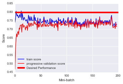
上图表明,在50次mini-batches滞后,分数提高就很少了,因此我们可以提前停止训练。由于训练分数和泛化分数差距很小,其训练分数较低,因此可能存在欠拟合的可能。
然而SGDClassifier不支持核技巧,根据图谱可以使用kernel approximation。
The advantage of using approximate explicit feature maps compared to the kernel trick, which makes use of feature maps implicitly, is that explicit mappings can be better suited for online learning and can significantly reduce the cost of learning with very large datasets. The combination of kernel map approximations with SGDClassifier can make non-linear learning on large datasets possible.
相较于核函数隐示的映射,kernel approximation使用显示的映射方法,这对在线学习非常重要,可以减少超大数据集的学习代价。使用SGDClassifier配合kernel approximation可以在大数据集上实现非线性学习的目的。
手写体数字识别
现在尝试对手写体数字问题进行建模。
可视化
1 | # http://scikit-learn.org/stable/modules/generated/sklearn.datasets.load_digits.html#sklearn.datasets.load_digits |
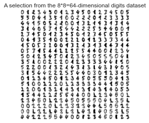
手写体数字的64维特征就是一个8*8数字图片每个像素点平铺开来的。因此我们可以通过上面代码进行重建图片。1
2
3
4
5
6
7print digits.images.shape #三维数组(1083L, 8L, 8L),1083个样本
print img.shape #二维数组(200L,200L),每个样本占8*8小分块矩阵。每8行20个样本,一共可以放400个样本。
#可以扩大该二维数组,例如(320L,320L), 每个样本占8*8小分块矩阵, 每8行展示32个样本,最大可以展示1024个样本。即32*32
# digits.images[0] == img[1:9,1:9]
# digits.images[1] == img[1:9,11:19]
plt.matshow(digits.images[1],cmap=plt.cm.gray) #第二个样本为数字1
plt.matshow(img[1:9,11:19],cmap=plt.cm.gray) #第二个样本数字1
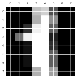
上述代码展示一个数字的结果,可以发现digits.images1和img[1:9,11:19]都是代表第二个样本,我们可以从图中看出第二个样本数字是1。
进一步可视化:1
2
3
4
5
6
7
8
9
10
11
12
13
14
15
16
17
18
19
20
21
22
23
24
25
26
27
28
29
30
31
32
33
34
35
36# Helper function based on
# http://scikit-learn.org/stable/auto_examples/manifold/plot_lle_digits.html#example-manifold-plot-lle-digits-py
# 我们之前已经讨论过手写数字的数据,每个手写的阿拉伯数字被表达为一个8*8的像素矩阵,
# 我们曾经使用每个像素点,也就是64个特征,使用logistic和knn的方法(分类器)去根据训练集判别测试集中的数字。
# 在这种做法中,我们使用了尚未被降维的数据。其实我们还可以使用降维后的数据来训练分类器。
# 现在,就让我们看一下对这个数据集采取各种方式降维的效果。
from matplotlib import offsetbox
def plot_embedding(X, title=None):
x_min, x_max = np.min(X, 0), np.max(X, 0)
X = (X - x_min) / (x_max - x_min)
plt.figure(figsize=(10, 10))
ax = plt.subplot(111)
# 绘制每个样本这两个维度的值以及实际的数字
for i in range(X.shape[0]):
plt.text(X[i, 0], X[i, 1], str(digits.target[i]),
color=plt.cm.Set1(y[i] / 10.),
fontdict={'weight': 'bold', 'size': 12})
if hasattr(offsetbox, 'AnnotationBbox'):
# only print thumbnails with matplotlib > 1.0
shown_images = np.array([[1., 1.]]) # 定义一个标准点
for i in range(digits.data.shape[0]):#样本数
dist = np.sum((X[i] - shown_images) ** 2,axis=1)#计算要展示的点和目前所有的点的距离,
#axis=1代表横着加,即每个样本x^2+y^2; 得到该样本和所有的点的距离的数组;axis=0,按列加,就变成了把每个样本的x^2全加起来,y^2全部加起来。
if np.min(dist) < 4e-3: #选择最近的距离
continue # don't show points that are too close
shown_images = np.r_[shown_images, [X[i]]] # 纵向合并
imagebox = offsetbox.AnnotationBbox(
offsetbox.OffsetImage(digits.images[i], cmap=plt.cm.gray_r),
X[i])#X[i]代表每个样本的两个维度的值,即横轴和纵轴的值,即两个维度决定的位置画出灰度图
ax.add_artist(imagebox)
plt.xticks([]), plt.yticks([])
if title is not None:
plt.title(title)
降维
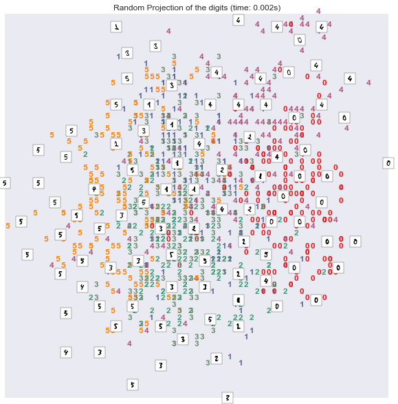
随机降维1
2
3
4
5
6
7
8#降维——随机投影
#把64维数据随机地投影到二维上
from sklearn import (manifold, datasets, decomposition, ensemble,
discriminant_analysis, random_projection)
rp = random_projection.SparseRandomProjection(n_components=2, random_state=42)#随机投影到两个维度
stime = time.time()
X_projected = rp.fit_transform(X)
plot_embedding(X_projected, "Random Projection of the digits (time: %.3fs)" % (time.time() - stime))
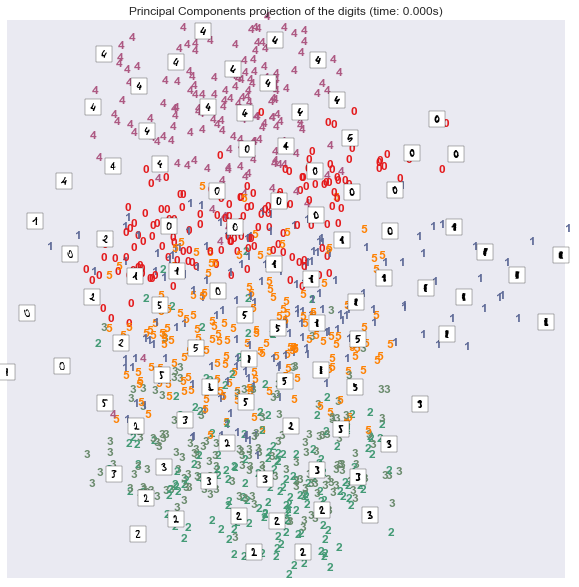
PCA降维1
2
3
4
5
6
7
8
9# PCA降维
# linear线性降维
# TruncatedSVD是pca的一种方式,不需要计算协方差矩阵,适用于稀疏矩阵
# PCA for dense data or TruncatedSVD for sparse data
#implemented using a TruncatedSVD which does not require constructing the covariance matrix
# LSA的基本思想就是,将document从稀疏的高维Vocabulary空间映射到一个低维的向量空间,我们称之为隐含语义空间(Latent Semantic Space).
X_pca = decomposition.TruncatedSVD(n_components=2).fit_transform(X)
stime = time.time()
plot_embedding(X_pca,"Principal Components projection of the digits (time: %.3fs)" % (time.time() - stime))
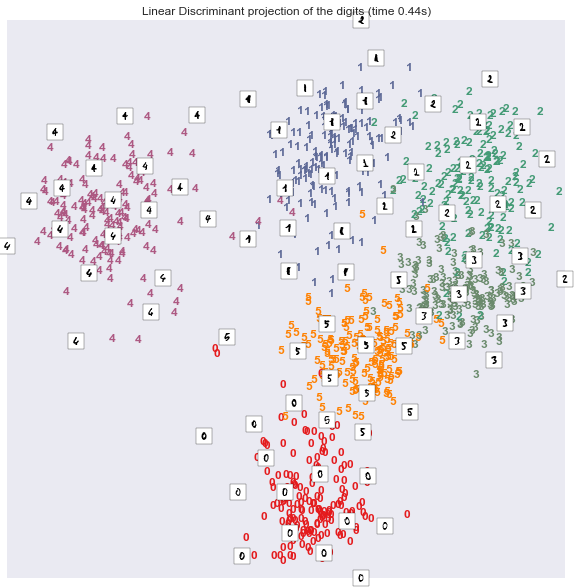
LDA线性变换1
2
3
4
5
6
7
8print("Computing Linear Discriminant Analysis projection")
X2 = X.copy()
X2.flat[::X.shape[1] + 1] += 0.01 # Make X invertible
stime = time.time()
X_lda = discriminant_analysis.LinearDiscriminantAnalysis(n_components=2).fit_transform(X2, y)
plot_embedding(X_lda,
"Linear Discriminant projection of the digits (time %.2fs)" %
(time.time() - stime))
t-SNE非线性变换1
2
3
4
5
6
7
8#http://scikit-learn.org/stable/modules/generated/sklearn.manifold.TSNE.html#sklearn.manifold.TSNE
#非线性的变换
#最小化KL距离,Kullback-Leibler
tsne = manifold.TSNE(n_components=2, init='pca', random_state=0)
stime = time.time()
X_tsne = tsne.fit_transform(X)
plot_embedding(X_tsne,
"t-SNE embedding of the digits (time: %.3fs)" % (time.time() - stime))
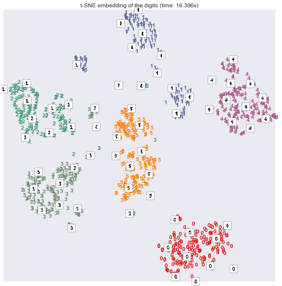
可以发现,在该数据集上,非线性变换的结果比线性变换的结果更理想。
损失函数选择
下面列出常用的一些分类损失函数。$y$的取值为1或-1。下图中,横轴是$yf(x)$,纵轴是损失值$L(y,f(x))=L(yf(x))$,分类损失是关于$yf(x)$的单调函数(而不是关于$f(x)$)。
1 | # adapted from http://scikit-learn.org/stable/auto_examples/linear_model/plot_sgd_loss_functions.html |
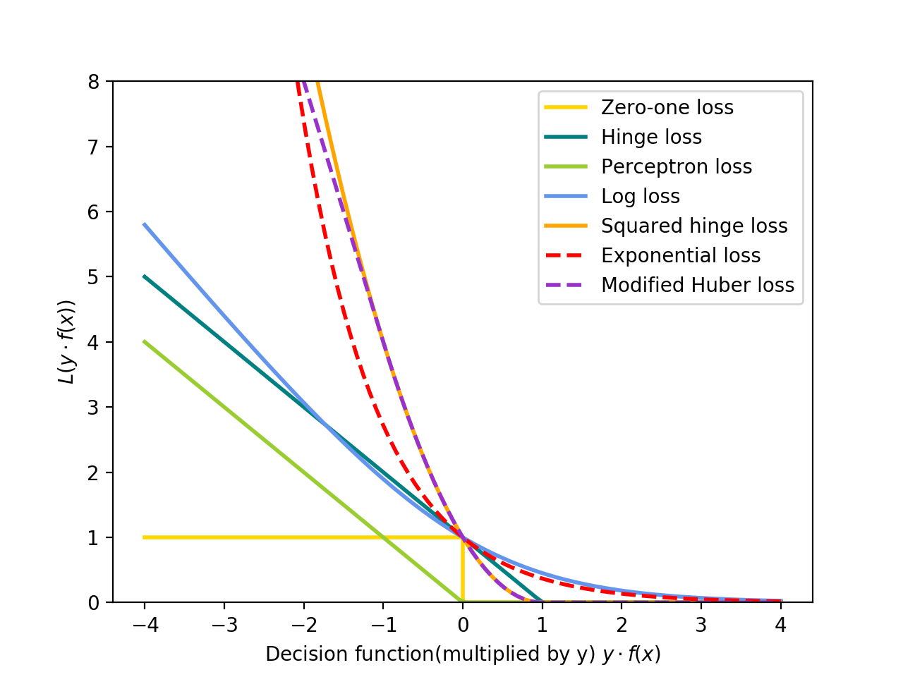
不同的代价函数有不同的优点:
0-1 loss: $\frac{1}{2}(1-\text{sign}(yf(x)))$,在分类问题中使用。这是ERM用的代价函数,然而是非凸的,因此必须使用其他代价函pr来近似替代。
hinge loss: $\max(0, 1-yf(x))$ 在SVM中使用,体现最大间隔思想,不容易受离群点影响,有很好的鲁棒性,然而不能提供较好的概率解释,又称为L1-Loss。
log loss: $\log(1+\exp(-yf(x)))$ ,实际上就是Sigmoid函数取负对数。在逻辑回归(和二分类交叉熵损失实际上是等价的,只不过那里y取1或0,这里y取1或-1)使用,能提供较好的概率解释,然而容易受离群点影响;
Exponential loss: $\exp(-yf(x))$,指数代价,在Boost中使用,容易受离群点影响,在AdaBoost中能够实现简单有效的算法。
perceptron loss: $\max(0, -yf(x))$,在感知机算法中使用。类似hinge loss,左移了一下。不同于hinge loss, percptron loss不对离超平面近的点进行惩罚。
squared hinge loss: $\max(0, 1-yf(x))^2$,对hinge loss进行改进,又称为L2-Loss,可微分,处处可导,(因为(1,0)处左右两边都可导,且导数都为0)。
modified huber loss: $\max(0, 1-yf(x))^2, \text{for} \ yf(x)\geq -1; -4 yf(x), \text{otherwise}$,对squared hinge loss进一步改进,是一种平滑损失,能够容忍离群点的影响(离群点损失的影响降低, 平方级损失变为线性的)
可以进一步参考:机器学习中的常见问题——损失函数
参考
斯坦福机器学习:Advice for applying Machine Learning
Advice for applying Machine Learning